This is my first blog post and I know this is going to be a long one, but I really really want to deliver the best content for the students who are enthusiastic about mathematics and want to learn how to solve these types of problems, which are not covered typically in schools or JEE preparation. I’d first like to list all the problems and then we will begin the discussion.
⚔️ Problems
-
The problem is in two parts.
a) Let be such that the straight line on the -plane passes through and . If are rational numbers with and , show that and are rational numbers and .
b) Let be such that and the circle on the -plane passes through , and . Assume that are distinct rational numbers, and are distinct rational numbers. Show that and are rational numbers.
-
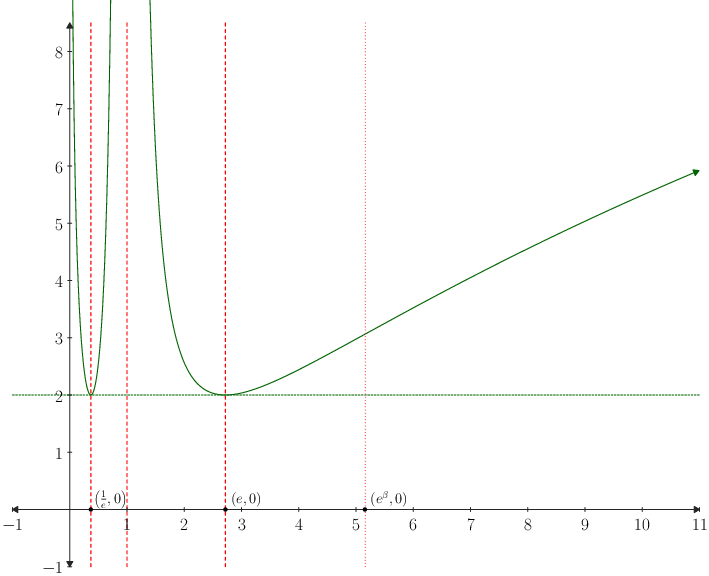
Sketch, with reasoning, the graph of .
-
Suppose is an integer. Define
and a function by
Determine the minimum value of over .
- Suppose is a twice differentiable function such that
a) If denotes the derivative of , show that
b) Further assume that , where is the second derivative of . Determine .
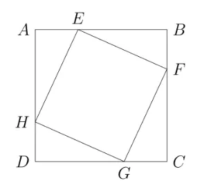
- In the figure below, is a square. The points lie on , respectively, such that is a square. The perimeter of exceeds the perimeter of by 32 units. Determine the length of the radius of the in-circle of .
-
Let be a polynomial of degree greater than or equal to one, with real coefficients, such that for all .
a) Suppose is such that . Show that there exist a positive integer and a polynomial with real coefficients such that and
b) Hence or otherwise, show that there exist polynomials and with real coefficients such that for all and
-
Suppose is a polynomial with integer coefficients.
a) Show that for distinct integers and , is an integer.
b) Hence or otherwise, prove that there do not exist distinct integers such that
-
Let be a non-negative integer.
a) Show that there exists a unique polynomial of degree with real coefficients such that
b) Determine the coefficient of in .
c) Hence or otherwise, determine the coefficient of in .
📌 Problem 1
We will start with part a). Since we know that and both lie on the line , putting these coordinates will satisfy the equation. This is simplest way to use the problem constraint. This gives,
where we know that all are rational. A very simple thought from here on, is to subtract the above equations. This gives . Clearly, we want to factor out the from LHS, to get
From here, if (this is actually true, since we are given that ), then we can divide both sides by and we would get . Well, is this fraction rational? If so, we would be done.
It turns out that its trivially a rational, the denominator since both and are rational. The denominator is non-zero as well, so we are really done! One needs to check the rationality of numerator of numerator as well, but well again, difference of two rational numbers is always rational! So, we have proven . What about ? Look at the equation . One can conclude that (find out how! its easy!) Let’s move to the next part.
Part b) has a similar flavour, it says there are three rational points(by rational points, we mean both coordinates are rational) on a circle. We are required to show that the center has rational coordinates as well.
A simple and naive way, could be to put , and back in the equation and then hope for something(maybe some cancellations like last problem ?) Before going too deep into calculations, we should look at the setup from a high level. We will call points and similarly define . We are given that the circle passes through 3 points, therefore its circumcenter is pre-determined. Therefore, if we try to mindlessly solve some equations, we should be able to extract individually.
It is obviously possible to put the coordinates of into the equation and bash out the values of and . But we will try to find a more geometric approach, which comes from the proof of the fact that three distinct non-collinear points on the plane has a unique circle passing through them.
Note that the perpendicular bisector of would pass through [the motivation to consider this, comes from the proof of existence of circumcircle of a triangle]. Similarly, the perpendicular bisector of would pass through as well. So, if we can write down the equation of the perpendicular bisectors then we can solve the linear equations in two variable, and we would be done!
Luckily, this is feasible. We can find the slope of perpendicular bisector of easily it is exactly
Note that the perpendicular bisector of will pass through , which is a rational point. If the equation of the perpendicular bisector is , then we already know , by putting the midpoint of , then we can find out , which will be rational(easy to see when you crunch the numbers).
The main discovery is that equation of the perpendicular bisector has both slope and -intercept both rational. If you solve both the equations, there is no way you get an irrational point! This concludes the problem.
📌 Problem 2
Ahh, I think this one is easily the most deceptive problem of the test and scoring full marks on this problem is going to be quite hard since there is quite a lot to do.
As you transition into higher math, you would usually use to denote the logarithm with base , but for this problem, we’ll use for the natural logarithm with base . We basically want to graph the function .
Personally, whenever you are attempting to make a graph of any function, you should do the following.
-
Determine the domain and range of the function .
-
Finding all the roots/zeroes of function or at least estimating them, if there is no nice closed form solution.
-
Find all it asymptotes, if there are any. Usually occurs when the denominator becomes , but there are other cases too. You can read more about it here on wikipedia.
-
Find all critical points of the function (a point is said to be critical if or isn’t differentiable at )
-
Find all the global and local maxima/minima of the function.
-
Monotonicity, find out the intervals, where the function is increasing or decreasing.
-
Convexity/Concavity, finding out the interval where the function is convex/concave(as an oversimplification, the sign of ).
Let us start with the domain and range. The domain is quite is easy, it is simply since has range and has domain , where we remove to keep the denominator non-zero. The range is slightly trickier, although with the aid of AM-GM Inequality on and (both are non-negative), you can at least see that for all in its domain.
Clearly, there are no zeroes of this function , which is quite easy to check. The vertical asymptote can only occur at and since these are the only points where the function collapses. It is easy to check that
which easily tells us the shape of graph of around the straight lines and . To check the critical points, we will now take the derivative of to find the critical points. The function is differentiable in its domain, so taking a derivative gives
Solving a simple equation from here, we will get that . Also, note that under ‘s domain
Since in our domain, we now need to solve . The neat trick(very standard though) is to multiply both sides by which is non-negative, so sign of inequality doesn’t change. This gives . From here, putting , this is a standard inequality to solve, which upon solving yields
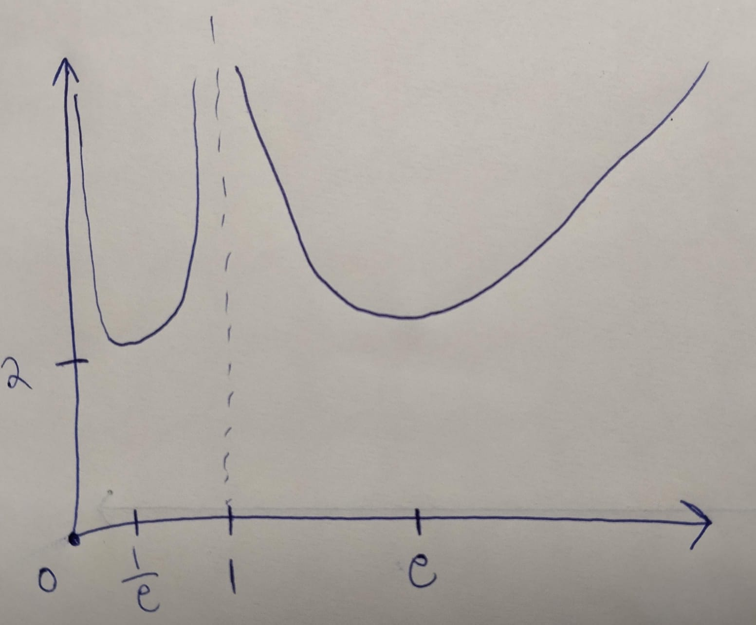
which basically gives us that is increasing over and . Also, from here we can conclude that decreases on and . With this information, applying the first-derivative test, we can verify that both at are global minima. At both the points , . With all these facts with us, let’s sketch a rough graph without considering the convexity.
Finally, lets evaluate the second derivative of . Differentiating we get(we’ll skip the details since its just a boring routine differentiation calculation)
where . Once again when is ? Multiplying both sides by , gives
Substitute , because we see a polynomial in . Finally, we need to analyze when . Call this polynomial . Note that this is the final part of the problem, we just need to figure it out when when positive or negative. Before doing anything, we should try to find out a few values of , like maybe , , and stuff, basically find out around , although we don’t really get much from it. With nothing left at hand, we will differentiate to find out nature of monotonicity of .
Even the derivative looks obscure… Trying a few values like might help… Oh! . So, with the division algorithm we get . Now, its quite clear that for . So, is increasing over . This is a LOT of progress at hand.
We do need to find the nature of on as well. Can we somehow get a handle on the roots of ? Let’s try differentiating this one, we would get … Can we comment on the sign of the derivative? Well, after completing the square or implementing any method of your liking, its very easy to see that this this is always positive! This means is always increasing! But this is a cubic polynomial, so it must have at least one root. Due to its strictly increasing nature, it must have only one root. I think before proceeing we should try to get an estimate. If we call , then , . Ah! The polynomial changes sign! So by the Intermediate Value Theorem(IVT), the root(call it ) must lie between and . So, by factor theorem
where is a quadratic polynomial. This quadratic polynomial can’t posses a root since only one single root. It can be either strictly positive or negative. By comparing the leading coefficient, one can easily say that must be strictly positive.
Analyzing the sign of the derivative is quite easy now. We now know that is strictly increasing over , we also know that , solving for we get that . So, is decreasing over . Before proceeding, we should make a rough-graph of .
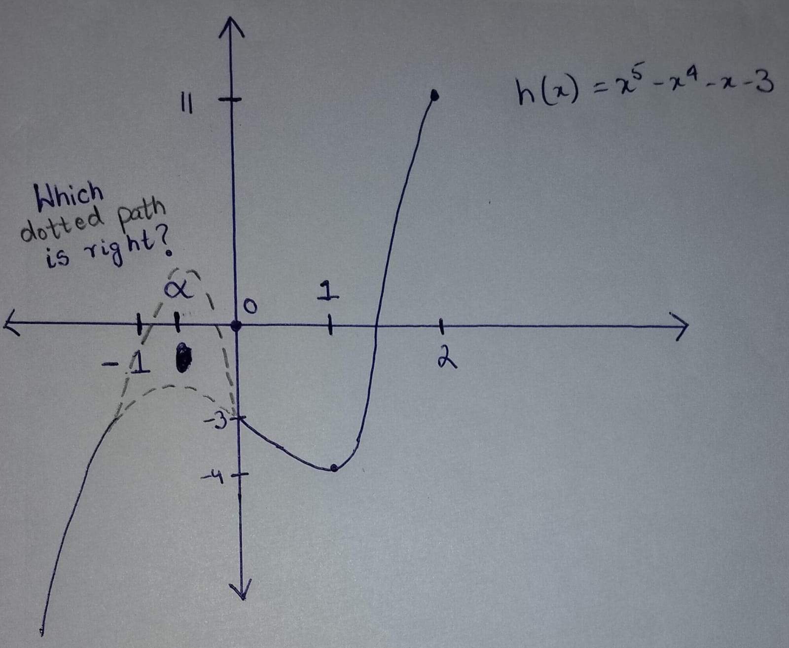
As you see can see above, we know and we know there exists some root of in . We also know there is a local maxima of around , but we are unsure whether or …
I’ll admit is blatantly. Beyond this point, I myself got stuck. I looked online, basically on YouTube. But what I found was, everyone hand-waved this part without paying much attention. I’d rather admit I wasn’t able to solve the problem, but I’m here learning stuff with you guys. Here’s a very magical claim, which I got by graphing on graph on Desmos and some AI asistance.
We will make two cases, whether or or . The case can be just checked by hand.
If , then . This gives . Then
This completes the proof to the first case. For the second case, assume . This gives and . Then
this concludes the proof.
Yes, I completely agree the above proof had almost no-motivation. The claim itself is quite hard to come up with without a computer/calculator. The proof itself is some algebraic manipulation which honestly is quite hard in the heat of examination, although it could be done. This indeed would take a lot of hit and trial to come up with the right bounds and thus I would not give any motivation for this, it only requires very standard inequality facts but its extremely ingenious!
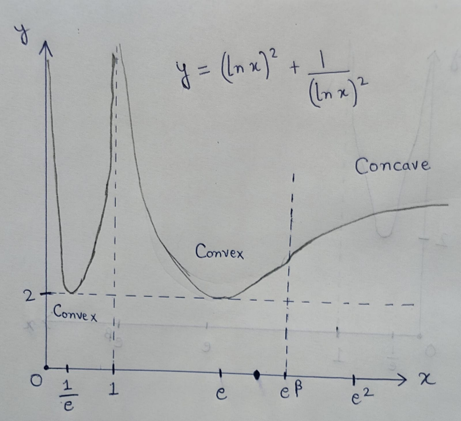
With this, we can now complete the graph of which we drew above and then we can finally conclude that is positive over and negative on . Also, do note that since and , with Intermediate Value Theorem(IVT) we can say that .
To finish it off, we know now that
Since is a continuous and monotonically increasing function, we can write
This finishes off the analysis for curvature and the solution. We’ll attach two images, one image will be hand-drawn for reference what to be drawn in exam and one is a computer-generated graph for fun!
📌 Problem 3
Okay, the notation might be a bit scary for some people. So, we’ll go bit slowly. The definition of set just says that we are storing all the ordered tuples of the form where every entry say strictly lies between and in the set . Then we define a function which takes input from and gives output in , basically we are given a function which takes multiple input values to give a single real output. Then basically you have to minimize the quantity
where every is between and .
At first glance, you just wonder what even is written here? The pattern is a little bit weird to write down. More concretely, how would you write this sum in a proper summation formula with with proper indexing and stuff? That’s quite a good question, which you might want to address.
Well, we will skip that question for now. Looking at the problem for a general looks scary, so we resort to first looking at small base cases to at least be able to see what is really happening here. We will start with . If you understood what the sum was written well, then you should realize that you need maximize
where . This looks like an optimization problem with just two variables. We can immediately see that we can just put write . The next step just needs the student to know a bit of logarithmic manipulation and I feel is quite standard if the student has spent at least sometime learning about logarithms. Basically, all I want to say is that quick change of base formula for logarithms, gives you that . Why would you do this? Well, you want all the logarithms to have the same base to make life easier and apply your standard logarithm formulas. We now just need to minimize
Minimizing these kind of things(by things I mean, something of the form where varies over ) is generally done using the AM-GM Inequality and this is a very standard method.
Although, here one needs to verify if is positive or not under the constraint that both lie in . Here’s a pretty cool thing, if is negative, then is also negative. So, even if these things turn out to be negative, we can apply AM-GM Inequality on and , although results will be different(can you guess what will be different?)
Anyways, if , then since is a decreasing function in (since ), we would get , which gives , which is just wrong since we are given that . So, safely applying AM-GM Inequality yields
So, we do have a lower bound! But, can the lower bound be achieved? Since we applied the AM-GM Inequality, the bound can be only achieved when
The above thing is only possible when you have . Well, can you find which satisfy the above equation? Its an equation with two variables, so naturally it should have an infinite number of solutions but the constraint on makes us question a bit whether there are enough solutions?
Since , so . So, if we just pick some , then must lie in . So, there exists plenty of . So, equality is achieved. The case was easy, what about ?
With , we want to minimize
This is much-much worse to deal with. Looking at it, I feel that after we solve this, we must be able to look at the true nature of the problem. Also, it is way better to transform all the logarithms into a common base. That way, if we want to apply our logarithm formulae, something like , then we can do it quite comfortably. We will keep the base , since it appears in the first summand. Applying change of base gives
This has kinda started to look like the previous case of . Would applying AM-GM inequality work? Actually, if you take the product of all the summands, you will find out that that the product is a constant. A perfect opportunity to apply AM-GM Inequality once again. It gives
Wonderful! We have a candidate lower bound with the help of the AM-GM Inequality. But if the equality is not achieved, then we can’t conclusively say that this is the minimium value. Once again, equality occurs iff
From here, we know , and . Multiply all these equations, to get . All of these are tactics a student should know, like if there is an equality with 2-3 signs, then letting everything equal to a common variable, in our case.
Here’s the final nail in the coffin. When there is the equality? We know that , so we may write . Here’s a crucial information, the moment you equated , you basically fixed the value of . Look at the summand , here when we set this thing equal to , then observe that we would get . The interesting part is that, once you try and set , you should realize that value of was already fixed. If the earlier value you found, doesn’t make , then there is no equality! Luckily, since . So, the equality holds, but what for what value of ? Well, recall you got the conditions and . These are the equivalent conditions for equality. Here, set to be some arbitrary number in , then we hope that and also lie in (yes they do! quite easy to prove). This finishes the case as well.
At last, I think we do need a definite pattern to state the equality case, how do we do that? We will do a general case this time, where we don’t fix a value of (feel free to try to get a better understanding of what is happening here).I think its fairly easy to see that the lower bound for a general with the help of AM-GM Inequality is . The equality occurs precisely when
where the last equality came from our trick of letting everything be and then multiplying equations, just like what we did in case. Even for this case, let . We firstly fix , then . Similarly, we can find that . If the student is willing to write down a few terms by hand, I think the pattern
for . Finally, pick some in , then will all lie in . This finally completes our solution.
📌 Problem 4
In particular, when someone wants to prove part a), then its quite natural to differentiate both sides, which is indeed valid, since is given to be twice differentiable. But, how do we even begin to differentiate? There are two variables! We have only learned to differentiate when there is one variable.
The given functional equation is true for all and all . So, lets fix for once. Then we would get
YES! Now, there is one variable, if we differentiate with respect to , we would get . But look at part a) again. It wants us to prove [because we put , so for now, we should be able to show this if the conclusion is true], which is something totally different.
Where did we go wrong!? A good observation is, to note that the functional equation, is not symmetric about and . Last time we fixed , this time let’s try fixing . This would yield,
Well, we can only differentiate this with respect to , so let’s do that. We get for all . Let’s go! This is what we wanted to show! We have just proven what we wanted to prove, but just for a special case when .
Here’s the fun thing, there is no such special thing while we take . We could have picked and would have gotten the same result! Therefore, we can directly say that if we differentiate both the equations with respect to (think that is constant and completely indepedent of ), then we get
which is what we wanted to prove! I think have explained it well-enough how this works out. People also call this partially differentiating with respect to . We will use the same terminology as well.
We now want to attack part b). This is much more interesting, since it wants us to characterize with an additional constraint that . As a student in exam, you might wonder why did they ask me to prove part a). You might want to use it. We were told the function is twice differentiable, we definitely want to use that to our advantage. We can differentiate both sides once again. But with respect to what? Well, if you partially differntiate with respect to , you get this complicated functional equation at the moment seems hard to deal with. It might be of use, but before committing to dealing with this monster, lets try and differentiate with respect to . We will get
I think with a little experience, one should know immediately what is happening. If you don’t, you can always manipulate. Just putting , gives . Replacing by in the newfound equation, we get for all . This is wonderful, the second derivative of is constant on entire . Just integrating twice, would yield
One still needs to determine the constants and . This can be done by blatantly putting this solution into the equation . We will take a smarter approach and try to play a little more with the setup. Like, just put , you will immediately find that , this immediately gives (!)
What if you just put and let be free in original functional equation? You’d get , which upon gives , which means is even. But and we just found out , can you now conclude that is forced!? This basically finishes the solution.
We have now found that for all . Although, as functional equations have this rule, that we must check whether the function which we have found is satisfying the functional equation. This is left as an exercise 😉
📌 Problem 5
A lot of the folks might just directly know the formula for in-radius of a right-triangle directly which makes the problems A LOT easier. I personally knew that too, but here is another approach, which comes from the formula where is the area of the triangle and denotes the semi-perimeter.

Let be the side-length of square . Then by the perimeter condition, we get that side-length of square is . We wish to compute the in-radius of . Applying the formula, we know that
Finding the area of triangle is quite easy, it is just . The semi-perimeter is just . We already see and appear twice, so let’s just label it for now. We will call and , with the usual naming conventions in . Now, we want to simplify
We for sure need some relations among the variables before we proceed for any computation. A very simple relation can be obtained by applying Pythagoras Theorem in , which gives . This kind of helps us get rid of completely(since we can put no matter how ugly it is), if we look at the expression completely algebraically.
Here’s the main meat of the problem. Look all the side triangles formed, basically , , and . They look quite similar on the diagram. I think one reasonable guess from the diagram, could be to claim they are congruent? Although, we have no clue if its true. We were never told that the given diagram is upto scale…
If you think this way of seeing the diagram and then claiming that these triangles are congruent can be done only if one knows the solution, then we’ll present another argument which is something you might find in exam. I do admit this is quite clumsy and I won’t like to present this in any formal solution, but maybe a more natural way to stumble around this congruency fact.
Let . We know that . Soo, . This also gives .

From here, I think one must be obervant to see that two right triangles with same hypotenuse length and a common angle , are they similar? Are they congruent? This isn’t anything super difficult, but yes one must be attentive all the time.
So, how do we prove that the triangles are congruent? Well, we know that . We also know that and . So, with basic class 9th standard AAS congruence rule, we get that . So, what information do we get? If you list everything out, the main information we get is that . Recall we had to compute
We now know that . So, everything simplifies into terms of . We just want to find the value of . We know that and . Simple algebra gives us that
We can now finally conclude,
which finishes our solution. The only challenging part of the problem was to notice the congruent triangles, which is quite doable even in exam conditions if just one calmly manipulates the expression they need to simplify. Although, I think it should have been clearly mentioned that the answer is a fixed real number, otherwise it can honestly leave a student very confused as to where to stop simplifying. The problem is easy because of the pre-existing formulae and like the main observation is not impossible because of the given diagram in the paper.
📌 Problem 6
This one is my favourite from the exam and I found it to be the most elegant problem in exam. We will start with part a).
Well, basically we have a non-negative polynomial where is a root of . What the problem asks you to show that any root of must come with an even multiplicity. There is quite a strong and important lemma for finding double roots which one must know before-hand.
Obviously, must have an even degree, otherwise its impossible for to be always non-negative. If you try to sketch a graph of , you’d immediately notice that attains at and then it must start increasing.
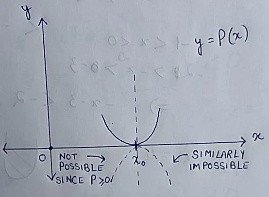
Similarly, must have been decreasing to before . This gives us that the LHD and RHD(these are right-hand and left-hand derivatives respectively) are and respectively. Since is a polynomial, the LHD and RHD must be the same. This is only possible if both are , which tells us that . From here, we definitely want to invoke our lemma and now we can conclude that is a double root of .
Well, so is a double root, so maybe we want to apply our division algorithm to get that there exists some polynomial such that
Wait, there is something interesting happening, if is not a root of , then we are done. We have shown that multiplicity of is 2(which is even), which is what we wanted. What if is a root of ? Well… We can try to apply a similar analysis as to what did before? Just if was also non-negative, we could have continued by factoring out more from … Wait, we know that for all and of course, for all ! This forces to non-negative on entire as well!
Well, since has finite degree, this must end sometime. We can easily see that is even degree, so everytime the degree decreases by . So, must have an even multiplicity, thus, we are done. Although, here’s an interesting and cleaner way to write this. What if we decided to induct on degree of ? The motivation for this, is simple. If didn’t have as a root, we would have been done, but if it had as a root, then we get a new polynomial with a smaller degree, where we have to do a similar type of analysis which we did earlier.
From here, its quite easy to conclude with induction. Although, the proof-writing needs real-care here. Its very easy to write a hand-wavy proof for the problem, which can lose points on the exam. Basically, this is what we want to prove in the exam.
Let . We wish to induct on . We first need to deal with the base case of . So, consider to have degree , with a root . By the Factor Theorem,
Soo, what we really want to show, is that also has the same root to prove our base case. Well, what if that is not the case? Well, if a quadratic has two distinct roots, then just graphing it out, one can see that it must be negative at some point of time.
Alternatively, say a quadratic looks like , where and , then just use wavy-curve method, you will always find a region where this quadratic turns negative. Therefore, two distinct roots are impossible for this quadratic polyomial, which proves that the hypothesis is true for the base case.
We’ll stop with the solution to part a) here, since the idea is now quite clear. Now one just needs to properly write down the induction hypothesis and induct properly with the equation .
We will now attack part b). This looks very very similar to part a). By the first part, we already know that if posseses a root , then we can write where . So, we have factored out one perfect square, and we know that is also non-negative. If posesses no more roots, then we are done! If it posseses one more root, say , then we can factor out that root with even multiplicity, and we would get
Once again, is non-negative. If doesn’t have any root, then its strictly positive and we would be done!
Sooo, yeah a similar induction argument like part a) will kill the problem here on the spot. This is almost the same as what we did earlier. So yeah, induction strikes again!
📌 Problem 7
Okay, I’m totally dissapointed by this problem. This is basically USAMO 1974/1. This problem is so common and almost anybody serious for the entrance must have solved this problem once before… Anyways, let’s see how to attack this.
So, we are basically given that (just a fancy notation for a polynomial with integer coefficients) and . Therefore, its quite obvious that and are all integers. Essentially, they want us to show that .
So, we are given has integer coeffcients. Well, the most straight-forward way to use this fact is to write down this polynomial. If , then
where are all integers. Let’s just compute what actually is. Obviously, cancels out.
So, now we just need to prove divides the RHS of the above equation. Obviously . Also, . So, can I in general say, ? If that’s true, we would be done! Well, there is a well-known identity
Since, are integers is obvious that the divisibility is true. This completes the proof to the first part.
Coming to part b), we wish to show there doesn’t exist such that some condition is true. So, just assume exists such that and . Ofcourse, we want to use part b). Lets try to use it. This would give us
Similarly with and , we will get the following division relations. This gives,
Obviously, none of none of them are , otherwise we get contradiction on distinct-ness of . If you look at these divisibility relations closely, then you would notice,
When is this even possible? Note that, we have a result that if , then given .
Applying the same result, we get that
Well, from here… You just need to show somehow that two of are equal, that will be the desired contradiction. Let’s start by crunching in some numbers,
because if two numbers have same absolute value, then they must be same or would be additive inverses of each other. If , then we get (contradiction, since , , are distinct). So, we get . With the other divisibility relations, we will similarly get
Just subtract any two equations. Magic will necessarily happen! The solution is now complete!!
📌 Problem 8
We will begin by part a). The biggest red-flag of this problem is sooo many god damn variables. You have and then … Nothing seems tangible at this point. I think a good way to start on this problem is to fix some variable. You definitely shouldn’t fix , because we are given that for all , this will vary throughout. You can definitely fix though. Lets try it out. Let’s start by fixing .
If we fix , then we get
for all . Does there exist some nice polynomial? Yes! It does exist! We know the formula for first natural numbers. We get which has exactly degree . Perfect! so, for there definitely exists a degree polynomial. Well, is it unique? Could there be any other degree polynomial which matches at all ? I don’t think I can motivate this one, this one should we known to the student prior to the exam. Consider the polynomial
where we have assumed is another polynomial where for all . If we can show that for all instead of just , then we would be done.
Here’s the magic! , and . So, as at least zeroes. But . This is impossible unless is the zero-polynomial!! This proves the uniqueness of the polynomial. We are done for case.
Well, obviously one would like prove this for I think we should try a few more examples. For , we again have a very good formula.
You can find out from here. Uniqueness can be proven once again! Just use that , which gives more zeroes. Well, has infintely many zeroes, you can handle uniqueness in genreal for any value of . You can try , you again have a good formula and you conclude for as well. There are good formulae for , but what are these? Would they remain of the polynomial type? Like, for , we get , which is a polynomial in . Are we sure that for , the formula would turn out to be a polynomial in ? If that is not the case, then everything collapses. We need to find a formal proof that this formula for is a polynomial in .
Writing down this proof, takes real experience and requires one to know their proofs. Do you know how to prove ? If you do, then the later steps are quite automatic, otherwise they are truly black magic. Note that
If you take a sum on both sides from to , then by telescopic sums, on the LHS you would simply get . The RHS becomes something much more interesting. Writing this properly we get
If you are observant enough, you just want to solve for on the RHS, rest all the formulae you already know! After simplifying, one would get
Which is again a polynomial. At this point, an induction (strong one to precise) on should be obvious since all you need is all the previous formulae. This indeed solves part a). But what about the other parts?
Well, okay lets think about part b) and part c) both at once, since both of them want us to find very particular coeffcients of the polynomial. First of all, if you just experiment with , you will out that the coeffcient of in is precisely for . So, its natural to conjecture that coefficient of in general is . Let’s try to justify it. Say you want to find a formula for , we will use the same telescopic black magic! We would then get
We know that we want to solve for . We know all the formulae for lower degree terms like , will only have terms of degree at most . Now, isolate to get
Notice that underbace, due to that logic, just find out the coefficient of from . It is precisely (!) Awesome, so if you cleverly add this to your induction hypothesis(since all you need is previous formulae) for part a), then you can solve part b) as well! Onto the final boss, part c).
There are two options from here, either you just extract the coeffcient directly from the above big equation with the underbrace, or you start slow and experiment a little with small values. Try out for , everytime the coefficient for comes out to be . Soo, we at least know now what should come after extracting coeffcient of in .
The underbraced part in , only has one term with , that is due to part b. By part b), we know the coefficient of in that term, must be . We can ignore the rest of the terms. The coeffcient of from can be easily found with the help of binomial theorem, its . So at last, the final coefficient of is
This finally concludes the solution. Phew, so many computations, it personally felt like a very long solution.
Technically speaking after assuming part a) and b), one can solve part c). And the inductive solution, should cover both part a) and part b) together.
Concluding Remarks
These are my final remarks on the problems this year.
- This first part of the problem is particularly easy and I feel it’s quite difficult to write a wrong solution. The second part is significantly more challenging, still if done correctly, even blatant computations can give a nice answer. There are several methods to solve this problem, one can even think of resorting to parametric coordinates for the circle, or bash it by putting values into the equation of the circle. This problem has appeared before which went as follows.
JEE Advanced(Subjective) 1997: Let be any circle with center . Prove that there can be at most two rational points on . A point is said to be a rational point if both its coordinates are rational numbers.
The taste of the problem is very similar and one who has done this problem beforehand can solve it almost immediately on exam. Regardless, there are quite a few approaches to consider, making the problem at a moderate level.
- I personally hate this problem. Finding the nature of the graph and the global minima and asymptote are typical of JEE Mains level these days. Any progress which just evaluates the derivative and finds the monotonicity of the graph is just routine calculation, which I feel should not be on the UGB section…
On the other hand, finding the curvature of the graph is stupendously hard. I personally don’t know how one is supposed to solve that inequality on exam, I think even showing that is concave and convex over certain intervals is quite hard! I would put the problem on the easier side of the exam, if the graders decide to give full marks to the people who have just decoded the monotonicity and asymptote of the graph. The problem easily becomes a hard level problem if graders penalize the students for not finding the curvature of the graph. Although, after searching through the internet, apparently a sketch of the graph doesn’t require you to find the curvature of the graph.
-
Ahhh! This one is an excellent trap for students. First the language of the problem might be a little intimidating; keeping that aside, attacking the problem with AM-GM inequality seems a reasonable approach (just because it’s one of the first inequalities a student learns and the case is quite motivating as well). The trap is and indeed the main meat of the problem is to determine the equality case. You just have to solve a few equations, although writing down details that the point at which minimum is attained indeed lies in is a little bit of a challenge, but an excellent problem to be asked on a subjective exam. In UGA settings, people might escape checking the equality case, but here working out the details is essential! This makes the problem easily at a moderate level, even a tiny bit on the difficult side.
-
A problem on functional equations, which has appeared after quite some time. If the student is familiar with the idea of partial differentiation, then the problem isn’t that difficult; you just have to differentiate twice and you are done. There is just a little hit and trial involved, which makes the problem very less involved.
The sad part of the problem is that similar problems have appeared in ISI 2019 as Problem 4, which were more difficult in nature. Moreover, I feel if someone has solved Cauchy’s Functional Equation over under the assumption that is differentiable, then we essentially have all the tools which we need. There are certain ideas, like making a form and then trying to force a derivative. This is quite involved, but can still be done if one really desires. Regardless, due to the direct and simpler approach, I would rate the problem as simple to moderate level.
-
Anybody experienced with even a little geometry experience, and knows the formula for a right triangle (right angled at ), then the problem becomes even more straightforward. Even bashing this out algebraically with is quite easy. This is clearly an easy geometry problem. I think this is quite an easy problem, with the only real challenge finding the congruent triangles, although this is quite easy because of the diagram drawn to scale. If not, then finding the similarity of the triangles is quite easy, from where congruency follows, as we covered in our solution. This problem is at an easy level, no matter how I try to look at it. The only problem could be a student’s inexperience with Euclidean geometry, but we can’t really do anything about it.
-
The double root lemma used here is extremely common and quite intuitive since we want to comment on the multiplicity of the root. It’s a little tricky to prove that , but once that is done the problem is straightforward via induction. Writing down a proper proof by induction is quite lengthy and details need to be written properly, but regardless the idea is quite easy.
There are other solutions to the problem, one is factoring via the Fundamental Theorem of Algebra and solving a few inequalities. I think that approach makes the problem more doable compared to what we have done in the blog (only because it doesn’t invoke the derivative lemma which we have used). This makes the problem quite doable. Anyways, I think the problem is around moderate level since writing a proper solution would take some time regardless of whether you factor or not.
- I can’t believe ISI could ask a USAMO 1974 problem directly on paper. It is not just that ISI is copying problems from the USAMO, but ISI copied the same idea from the UGA paper. The problem reads as
UGA 2026: Let be a polynomial with integer coefficients of degree greater than or equal to . Suppose and are both odd integers. Then equals
(A) (B) (C) (D) or more
The answer to the UGA problem is just . Assume there is any root of , then its quite easy to see is odd. Then by the part a) of the UGB Problem 7, we get . Now, is even but is odd! Contradiction!
The first part is extremely easy, no doubt about it. Just writing down the identity of is enough. The second part is indeed harder and one common mistake a student could commit is to use the false statement that
Instead, . This is the only mistake a student can make sitting in the examination hall. So, only due to this pitfall, I would rate the problem around easy to moderate problem.
- This was easily the hardest problem on the test. You need to know your proofs for the formula of and higher powers. Otherwise tackling the problem becomes difficult and requires more unorthodox thinking in the exam. One possible solution is via Riemann sums, which I might consider adding someday later in this blog, but that requires even more technical background before the test. This makes the problem clearly quite hard.
This problem even tests the student’s mathematical maturity by proving the uniqueness of the polynomial. Just seeing as a polynomial in doesn’t really finish the problem; you must show that the polynomial agrees everywhere on , not just on the naturals. The trick to doing this is extremely common, as Mr. KD Joshi says, defining a polynomial as and arguing that there are infinitely many roots of is important and quite a common idea in JEE Advanced.
Writing down a formal solution, which is not all over the place, is quite difficult and managing the calculations is also very important for this problem. This problem is an excellent problem, although too lengthy and tedious for my taste to appear on the test.
Brief Discussion on Cutoff
The cutoff for B.Stat Entrance 2026 has been declared on 11 June, 2026. One can see the entire Merit List.
UGA Cutoff declared is 63 and . Thus we can say a bare minimum to qualify the examination is 15 problems in the objective section and 4 problems in subjective section. The quality of UGA was very good this year and I feel if one picked the right problems from the UGA, one could have made a much better UGB paper.
There were a few notable problems in UGA which should have been placed on the UGB section instead of wasting the problems in UGA. I personally don’t understand why would the problem setting committee set such an easy UGB paper after removing the interview process.
The cutoff of 4 problems for UGB is totally reasonable since the UGB was much more doable. UGA was much harder and the student had to solve quite a lot of challening problems without too much break. I very avidly support the subjective section of the paper, but I feel UGA section was much more worthy of getting a higher cutoff because of the paper quality.
Final Comments
This year the paper quality has degraded once again compared to 2025 UGB. UGA quality has increased which I really appreciate. The problems were approachable with very simple techniques. The only notably good problems were Problem 1 part (a), Problem 6 and Problem 8. Problem 2, despite not being hard, is a very good problem for the subjective UGB section. I hope next year we could see a few interesting problems.
I really think ISI should stop copying problems like Problem 7, which are such a common illustration for anybody learning integer polynomials. Problem 2 and Problem 5 should be stated a bit more concretely: Problem 2 should have told what details they want in the graph and Problem 5 should at least mention if the answer is a fixed constant or not. It helps the student know much better what the grader is expecting, since there is no communication from a grader to a student at the time of the examination. Here’s a PDF with the correct and formal solutions to the problems.